Modern machine learning solutions have found their way in a plethora of scientific and technological advances and have by now reached millions of users. Several of these advances are made possible through state-of-the-art predictive models, equipped with hundreds of millions of trainable parameters. Training these enormous models can be a daunting task. For example it can take several days to train a deep learning model to state-of-the-art accuracy, even on high-end GPUs. Researchers and practitioners don’t always have that kind of time: sometimes we want to quickly test an idea that often requires retraining a model, and there may be hard time constraints for shipping trained models to production. It is natural to ask if we can speed up this process by leveraging 10s or 100s of GPUs in parallel. It turns out that scaling up model training is harder than it might seem. In this post, we explore the reasons behind it and suggest paths towards scalable training that have the potential to reliably work out of the box.

Background

Before we dig deeper into distributed training, it is worth highlighting some points of difference when comparing to more traditional compute tasks. Say for example that you’d like to accelerate a matrix vector operation A*x using 10 compute nodes. A straightforward approach to scale out across 10 nodes would be to slice A in 10 row-blocks A₁ … , A₁₀, and then assign to node i the computationally 10-times lighter task to compute A_i*x. Once nodes compute these smaller matrix-vector products, they can communicate and combine the local results to form A*x, i.e., the desired end result. More sophisticated variants of this simple approach can lead to nearly perfect speedups compared to computing A*x on a single machine. This is possible because distributed multiplication enjoys several attributes: it requires only a single communication step between compute nodes to combine local results, an exact solution can be computed with a “single pass” over the entries of A, and there are no major hyperparameters that require tuning.

By contrast, modern deep learning model training with an optimization scheme like stochastic gradient descent (SGD)—the workhorse of machine learning—lacks these attributes.

As we explain below, SGD requires hundreds of passes over the data that are communication heavy, and a multitude of hyperparameters to be fine-tuned for state-of-the-art performance.

Communication Bottlenecks

During each iteration of distributed SGD, each compute node samples a subset of training data points (i.e., a mini-batch), and for each data point computes a gradient with respect to a prediction loss on the current model. Each of these gradients is a direction of descent that when applied to the model improves its prediction loss with respect to the corresponding sampled data point. The batch of computed gradients is then aggregated using a synchronization step either in a distributed key-value store, i.e., the parameter server, or across compute nodes through a gather, or reduce-type operation, and is then applied to a shared global model. Note that the size of each of those communicated gradients is proportional to the number of weights of the trained model. SGD usually requires more than hundreds of passes over the data to achieve state-of-the-art accuracy. This translates to thousands or millions of distributed iterations. All this renders distributed SGD fantastically more communication intensive than vanilla matrix multiplication, as it requires many iterations during which billions of floats are communicated over the network of compute nodes. The dream of out-of-the-box distributed speedups is further cut short when the above are combined with the huge diversity of training tasks, model architectures, and intrinsic system bottlenecks not manifested in single machine implementations.

To address communication bottlenecks it is important to understand why they are seemingly inevitable as we try to scale out training to a large number of machines. Communication becomes a higher-order cost when aggregating gradients becomes more expensive than computing them. The communication cost of each distributed iteration depends on the different aggregation protocol used (e.g., ring-reduce), but let us assume the best case scenario where it is fixed with the number of machines. The per-machine compute cost is the amount of work (e.g., mini-batch) divided by the number of machines. Thus, as the number of machines grows, communication costs increase and per-node computation costs decrease leading to communication bottlenecks. While it is possible to increase the amount of work per distributed iteration by increasing batch sizes, such techniques are model specific and have been shown to have limitations.

Reducing the Flow

How do researchers deal with these bottlenecks? The research community has explored a wide range of approaches towards overcoming communication overheads, mostly focused on compressing or quantizing gradient updates in a theoretically principled way. Some examples of gradient compression or sparsification techniques include QSGD, TernGrad, signSGD, and ATOMO. In all these studies, once a gradient is computed, each node has to come up, on the fly, with an appropriate quantization or sparsification rule of gradient weights, or low-rank factors, in order to preserve only what is “important” while discarding the rest. Such methods can reduce communication costs by orders of magnitude, while not significantly hurting convergence performance. Unfortunately, several of these methods require additional compute for each iteration’s sparsification rule, may introduce more hyperparameters that require tuning, and focus on aggregation setups that have become less prevalent in practice, e.g., the parameter server, while being incompatible with all/tree/ring-reduce protocols that are widely used in industrial systems. Finally, most of these methods target a fixed, non-changing learning and system setup.

The practical value of any distributed training approach hinges on its amenability to be used out-of-the-box across a range of problems and setups, as opposed to its ability to be optimized for a specific workload and benchmark. Benchmarks like MLperf and DAWNBench have shown us that we can go from training an ImageNet model in 14 hours on a single P3 GPU to 1.3 minutes using hand-optimized distributed training strategies. This incredible 50,000-fold speedup requires hundreds to thousands of high-end GPUs, and months of human hours to hand-tune training hyperparameters that can many times be different across iterations and even compute nodes. Coming up with theoretically sound solutions for scalable distributed training that work out of the box on new problems may of course not be entirely feasible, as there is no silver bullet due to scalability depending on datasets/learning tasks/system setups. However, there are some simple design choices towards scalable training that can work well out of the box.

Optimizing Communication in Practice

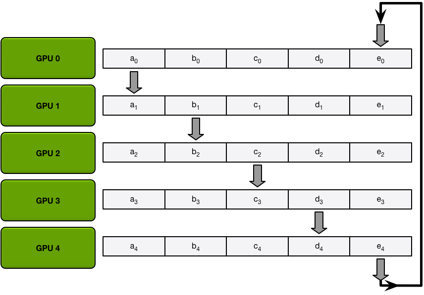
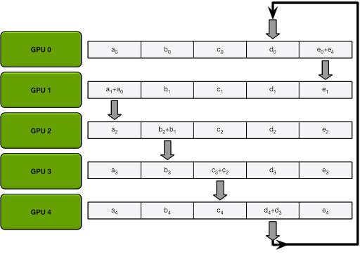
One design choice that works well out of the box is shifting gradient averaging from all-reduce/all-gather aggregators to ring-reduce, which has been popularized by tools like Horovod. In ring-reduce, the gradient is split into consecutive blocks at each node, and in-parallel each block is then pushed to the next node following a ring order, until every node has the sum of all gradients computed by the nodes.

This simple reduction strategy, unlike the parameter server, or all-reduce, can be shown to provide significant benefits as it offers a fixed communication cost independent of the number of GPUs used for training. Ring-reduce of course presents some latency bottlenecks that require more sophisticated solutions if we’d wish to scale out to thousands of GPUs, but this setup may be less relevant for the vast majority of training tasks and system setups.

Beyond Optimal Communication

To further limit the communication overhead of gradients, one has to come up with compression/sparsification techniques that are compatible with ring-reduce. To achieve this we have to narrow down the design space of methods to those that obey a certain “linearity” condition, where the sum of compressed/quantized gradients has to be equal to the compressed/quantized sum of the original gradients (i.e., the compression function has to become reduce-compatible). Certain sampling techniques that simply keep the largest gradient weights, or most prevalent low-rank factors abide to this requirement, while further reducing communication costs significantly. An important characteristic of these “simpler to implement” methods is that unlike QSGD, TenGrad, and signSGD (discussed earlier), they become adaptive to the training task and model at hand by following some simple rules. One way to accomplish this is by requiring that the compressed/quantized gradient is within small distance from the uncompressed ones, and by implementing system checks that measure the compute vs communication time per iteration in order to identify the appropriate amount of compression required. A key takeaway from our solutions that we ship in production is that they are robust, as they allow for adaptivity that renders them amenable for out-of-the-box deployment. We would like to conclude with noting that although distributed training is not trivial to scale, robust solutions that work on a wide variety of tasks can have a big impact, as they require minimal fine tuning for each independent learning task, making it easier for the end user to implement and test.

At Determined AI, we are actively experimenting with many of these types of optimizations in our core product. Importantly, by separating model definition from the optimization logic in our abstractions, we can experiment with many of these optimizations and turn them on/off if they make sense all without modifying user code. This means that the power of future, well-vetted research advances can be baked into the system over time.

In our next post in this series, we’ll discuss this in more depth.