SEP 11, 2024
Finding the best LoRA parameters


September 11, 2024
Introduction
While LoRA (Low-Rank Adaptation) is now widely used to fine-tune large language models, practitioners often have questions about its proper configuration. For example, an internet search for “how to set in LoRA” reveals conflicting recommendations. Some suggest that should be twice the rank, while others argue that should equal the rank, or even be half of it. Additionally, there are opinions that should remain constant as rank varies, as the original LoRA paper did.
In this blog post, we’ll offer evidence-based practical tips on setting important LoRA parameters for better training performance.
tl;dr
First, for those who prefer a direct recommendation, we recommend the following workflow if you are using an Adam-style optimizer:
-
Start with an arbitrary and rank of your choice, and tune the learning rate. Some libraries (e.g. Transformers) provide a default value for . If a default is not provided, simply set to be equal to the rank, as suggested in the original LoRA paper.
-
Once you find a satisfactory learning rate, adjust the rank as needed. There is no need to change the value; you can continue using the default from the first step.
Background
LoRA is a parameter-efficient fine-tuning method. Instead of updating the original weight matrices of a model, LoRA adds learned low-rank matrices to the frozen original matrices. This approach significantly reduces the resources required for fine-tuning, and speeds up the process, as the low-rank matrices are much smaller than the original matrices.
Before we go further, let’s recap the definition of rank and .
Rank
LoRA approximates the parameters of a large matrix, , by decomposing it into the product of two smaller matrices, and . The rank is the inner dimension of these smaller matrices. A higher rank requires more computational resources, but allows the model to capture more information, which can improve performance.
Alpha
During the forward pass, the output, , of a LoRA block is:
where is the frozen original matrix, is the rank of and , is the input to the block, and is a scaling factor that controls the degree to which and affect the output.
Experiment 1: Initial Run
Set-up
We conducted a series of fine-tuning experiments using the mistralai/Mistral-7B-Instruct-v0.2 model and the Clinton/Text-to-SQL-v1 dataset. Specifically, we used a “hard” subset1 of the data to capture more variance in the results.
In these experiments, we varied the and rank values while keeping other factors constant:
-
: [0.5, 2, 8, 32, 128, 256, 512]
-
rank: [2, 8, 32, 128]
-
rsLoRA: No
-
Learning rate: 1e-5
-
Optimizer: AdamW
This resulted in 28 training runs, each corresponding to a unique combination of and rank.
Observation #1
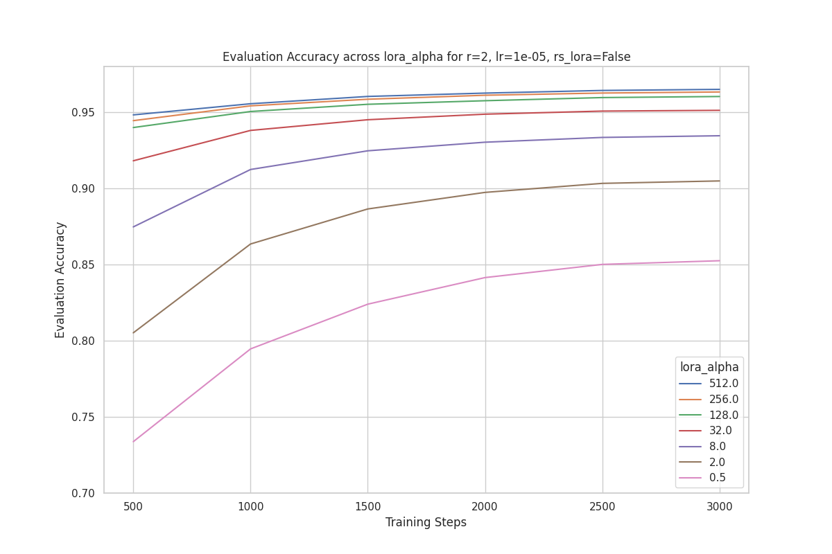
We observe that runs with a higher perform better for a given rank. This observation holds across all the ranks we experimented with. For example, the plot below is the evaluation accuracy with rank = 2 across different values. The best run uses .
Similarly, the plot below shows the evaluation accuracy with rank = 128 across different values. Once again, we can see that the best performing run is with .
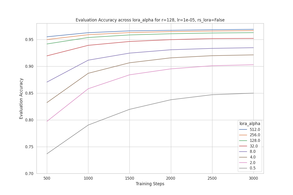
Based on the results above, we did not find any evidence supporting the claim that should be a specific multiple of rank or that it should vary with rank.
Observation #2
One perplexing observation is that for a given , there is no significant performance improvement as rank increases.
For example, the plot below shows the evaluation accuracy for runs with , where each line presents a training run with a different rank () value. As you can see, the performance differential is quite small across ranks.
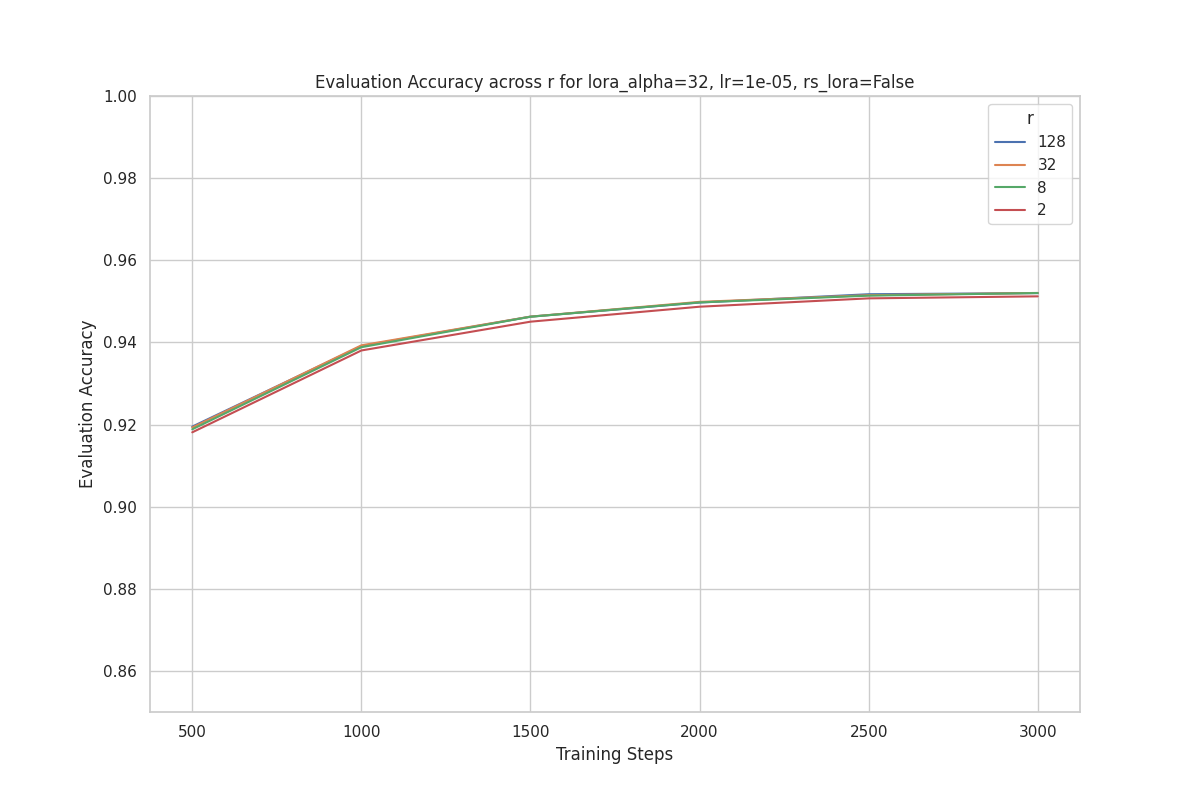
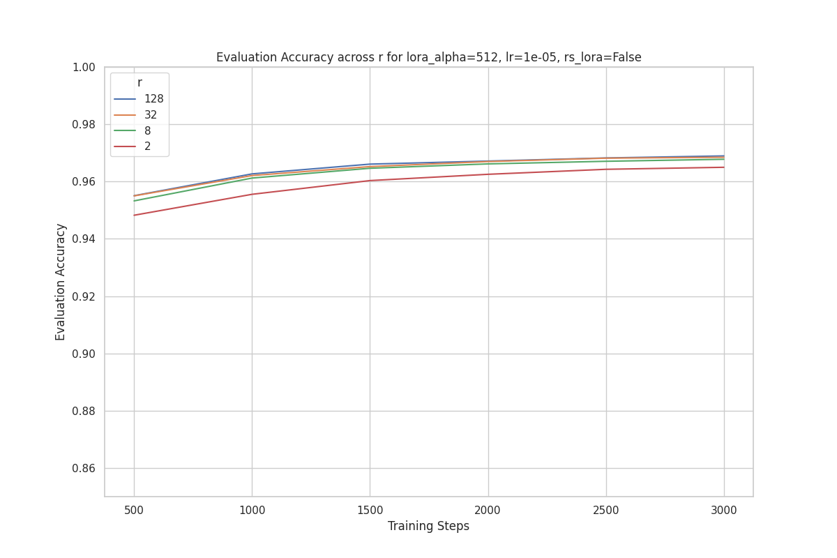
This clustering pattern is observed across different values of .
For example, below is the plot for .
These results suggest that the dataset and task are not very challenging for our model, because even with , the model is able to achieve high accuracy.
Next, we will present results of follow-up experiments addressing the two observations above.
Experiment 2: Alpha and learning rate (investigating observation #1)
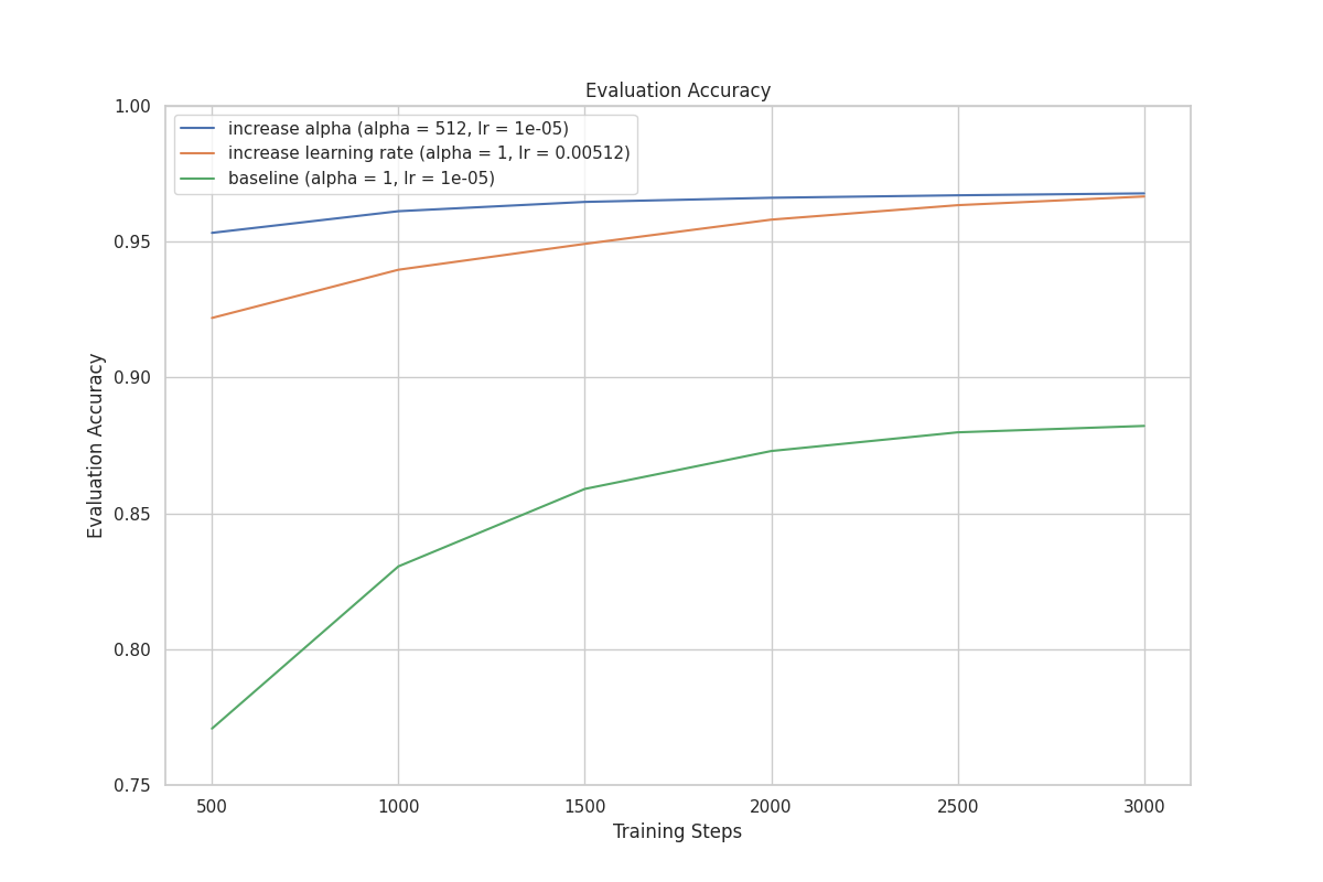
The LoRA paper states that “When optimizing with Adam, tuning is roughly the same as tuning the learning rate if we scale the initialization appropriately.”
Consider two training runs. Run Y has an value 512 times greater than Run X, and Run X has a learning rate (lr) 512 times greater than Run Y. As a result, their effective learning rates and performance should be similar. Our experiment results confirm this, as shown in the graph below.
| rank | lr | ||
|---|---|---|---|
| Run X | 8 | 1 | 0.00512 |
| Run Y | 8 | 512 | 1e-5 |
Experiment 3: Rank-Stabilized LoRA (investigating observation 2)
What still perplexes us is why, when and the learning rate are held constant, varying does not lead to a meaningful performance improvement, nor faster convergence. A review of related literature led us to a paper that proposes rank-stabilized LoRA (rsLoRA). The author finds that the scaling factor of is too aggressive, leading to gradient collapse as the rank increases. Instead, the author proposes a scaling factor of .
You can use the rsLoRA scaling factor with the PEFT library by simply setting the use_rslora option in the LoraConfig to True.
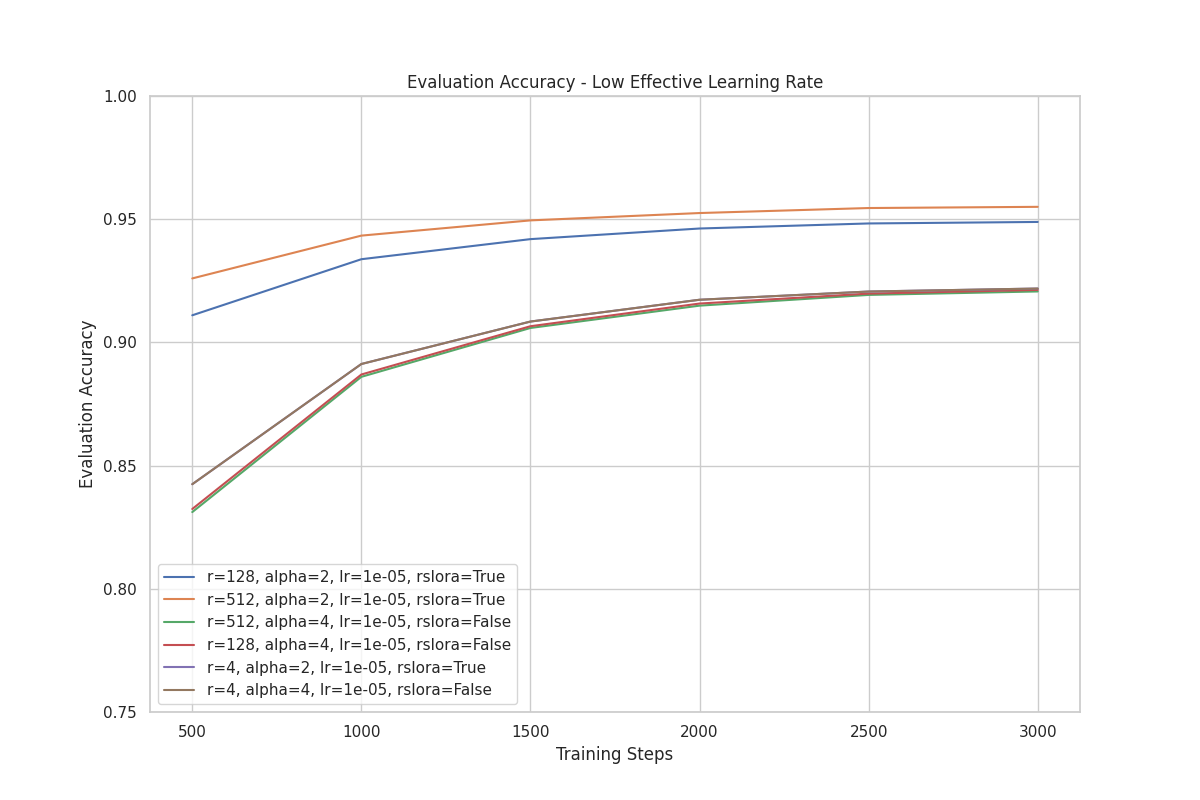
For these training runs, we started with a baseline where LoRA and rsLoRA use the same rank, and also perform the same (by ensuring that their scaling factors are equal):
- rsLoRA
- r: 4
- : 2
- Scaling factor:
- learning rate: 1e-5
use_rslora:True
- LoRA
- r: 4
- : 4
- Scaling factor:
- learning rate: 1e-5
use_rslora:False
Then we varied the rank in subsequent training runs, while keeping all other parameters unchanged.
In the plot below, we can clearly see that performance improves as rank increases when using rsLoRA.
We also conducted another experiment with a higher effective learning rate.
Like the previous set of training runs, we also started with a baseline where the performance of LoRA and rsLoRA are the same:
- rsLoRA
- r: 8
- :
- Scaling factor:
- learning rate: 0.00064
use_rslora:True
- LoRA
- r: 8
- : 8
- Scaling factor:
- learning rate: 0.00064
use_rslora:False
Then we varied the rank in subsequent training runs, while keeping all other parameters unchanged.
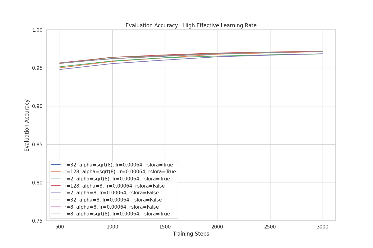
With a higher effective learning rate, the difference in performance between rsLoRA and LoRA is minimal. Additionally, we do not observe the same separation of performance when varying ranks for rsLoRA as we did in the previous set of experiments.
Diving deeper into the scaling for rsLoRA and LoRA, we see for :
- LoRA’s multiplier is
- rsLoRA’s multiplier is
And for :
- LoRA’s multiplier is
- rsLoRA’s multiplier is
Despite the differing multipliers, we see similar results for rsLoRA and LoRA at the extremes of . We think this could be caused by the loss surface having relatively wide minima that are easy to enter and stay within. It is likely we’ll need a more complex and difficult dataset to show the differences between rsLoRA and LoRA as we vary .
Conclusion
Given the above results, we suggest the following:
-
Start with the default and a rank of your choice, then tune the learning rate.
-
Once you find a satisfactory learning rate, adjust the rank as needed. There is no need to change the value; you can continue using the default from the first step.
In our experiments, rsLoRA did not help with model performance or hyperparameter tuning. For more difficult training scenarios where rank has a greater affect on accuracy, it is possible that rsLoRA provides some benefit.
If you’d like to run some LoRA experiments for yourself, check out our code on GitHub.
Appendix
Why is the scaling factor needed? According to the LoRA paper, “this scaling helps to reduce the need to retune hyperparameters when we vary ”.
Assuming we have identified a suitable learning rate for a specific value of , increasing will generally increase the vector norm of the LoRA adapters. This can lead to unstable training because the optimizer might overshoot with the same learning rate.
To avoid the repetitive task of tuning the learning rate each time is adjusted, a scaling factor is introduced. The purpose of this scaling factor is to maintain stable training across different values of . Specifically, as increases, the scaling factor decreases, which effectively reduces the learning rate for Adam-type optimizers.
This approach mimics the effect of adjusting the learning rate directly, thus preserving training stability without requiring constant manual tuning of the learning rate.
-
The hard subset we created consists of SQL queries with lengths between 201 and 800 characters. ↩