Here’s what caught our eye last week in AI.

1) Stable Video Diffusion

Stability AI has released Stable Video Diffusion, a new open-source video generation model. Included in the release are the weights and code for two image-to-video models that can generate 14 or 25 frames at a resolution of 576x1024, given an initial frame. The paper also describes a yet-to-be-released text-to-video model.

Here’s how they trained this new model:

1. Image pretraining on a large dataset of images

For this step, they started with a pretrained Stable Diffusion 2.1 model.

2. Video pretraining on a large dataset of videos

To make the dataset amenable to training for video generation, they used various heuristics to remove scene cuts and fades. Since the goal is a text-to-video model, they created multiple text descriptions for each clip, using an image-captioning model, video-captioning model, and an LLM that summarizes the output of the captioning models. The result was the “Large Video Dataset” (LVD) which contains 580 million annotated videos, 212 years in length.

However, the quality within this dataset varies significantly. To be able to find and filter out low quality videos, they added:

• Optical flow scores, to find long static scenes.
• Text detection scores, to find frames with lots of text.
• Aesthetic scores based on CLIP embeddings, to find visually unappealing frames. They seem to have used the LAION Aesthetic Predictor model which is built on top of CLIP.

Using these scores, they filtered out low-quality videos to obtain a new dataset (“LVD-F”) containing 152 million videos.

3. High-quality video finetuning

The final step was finetuning on a dataset of 1 million higher quality, higher resolution (576 × 1024) videos.

See some example generated videos here.

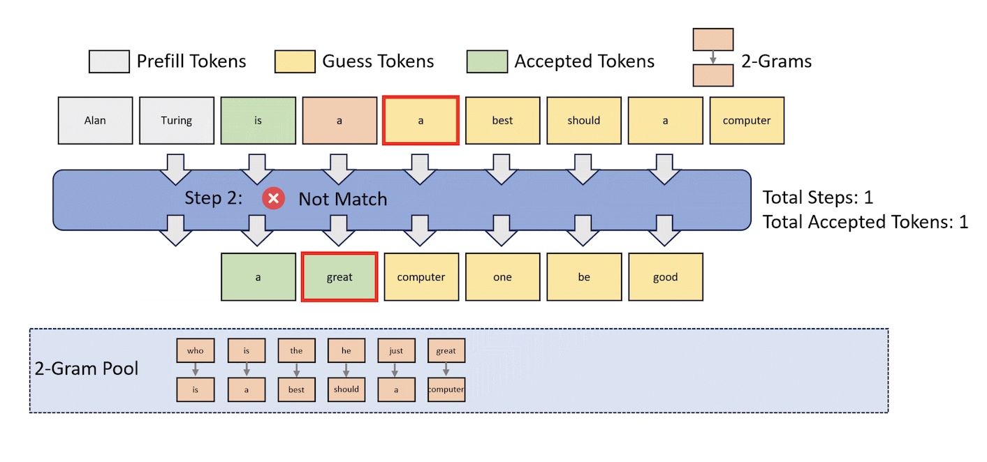
2) Lookahead Decoding

Everyone wants faster LLM responses, and there have been various ways to accomplish this, like:

• Speculative decoding^{1, 2}, which requires a smaller “draft” model that tries to predict ahead of the main model.
• Medusa³, which works similarly to speculative decoding, but uses additional finetuned layers rather than a separate draft model.

Lookahead Decoding is a new technique that speeds up LLM responses, without relying on additional models or layers. It builds off of a previous method called Jacobi Decoding, which itself is based on a commonly-used linear algebra algorithm. For a detailed explanation, see this blog post.

3) ZipLoRA

LoRA (Low Rank Adaptation) is a popular method for finetuning large models in a memory-efficient way. Finetuning a model this way results in a small number of learned parameters that can be swapped in and out. For example, you could use LoRA to finetune a model on pictures of dogs to obtain a set of parameters P_dog, and finetune the same model on paintings of flowers to obtain another set of parameters P_paintings. Then to create high-quality dog pictures, you would load in P_dog, and to create high-quality flower paintings, you would load in P_paintings.

But what if you want to create paintings of dogs. Is there a way to combine the capabilities endowed by both P_dog and P_paintings?

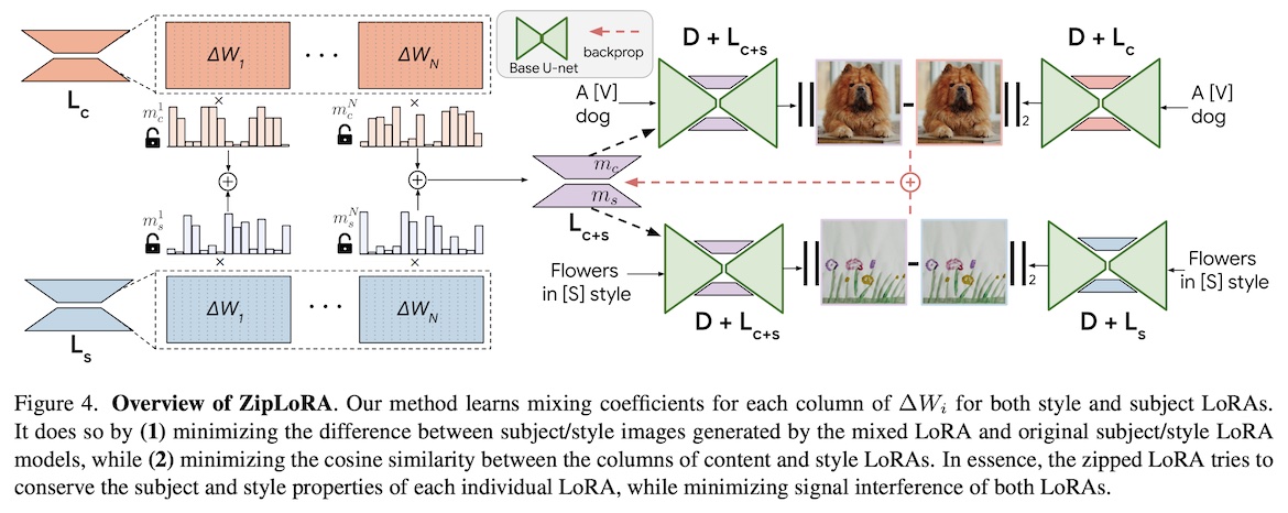
ZipLoRA is a new method that promises to do this. At a high level, it takes two sets of LoRA parameters (let’s call them P_c and P_s) and adds them together to obtain a new set of parameters P. However, simply doing P = P_c+P_s causes subpar results, because the subtleties in each parameter set is lost. To avoid losing these details, ZipLoRA instead does P = m_c⊗P_c+m_s⊗P_s, where m_c and m_s are learned multipliers, and ⊗ represents an element-wise multiplication. The multipliers are optimized such that:

• The images generated by P are as close as possible to the images generated by P_c and P_s. In other words, the goal is to not lose any of the capabilities of P_c and P_s.
• m_c and m_s have a low cosine similarity, i.e. they have as little “overlap” as possible. In other words, the goal is to emphasize complementary parameters of P_c and P_s, rather than parameters that “clash”.

Take a look at some sample outputs here.

Stay up to date

Interested in future weekly updates? Stay up to date by joining our Slack Community!