Introduction

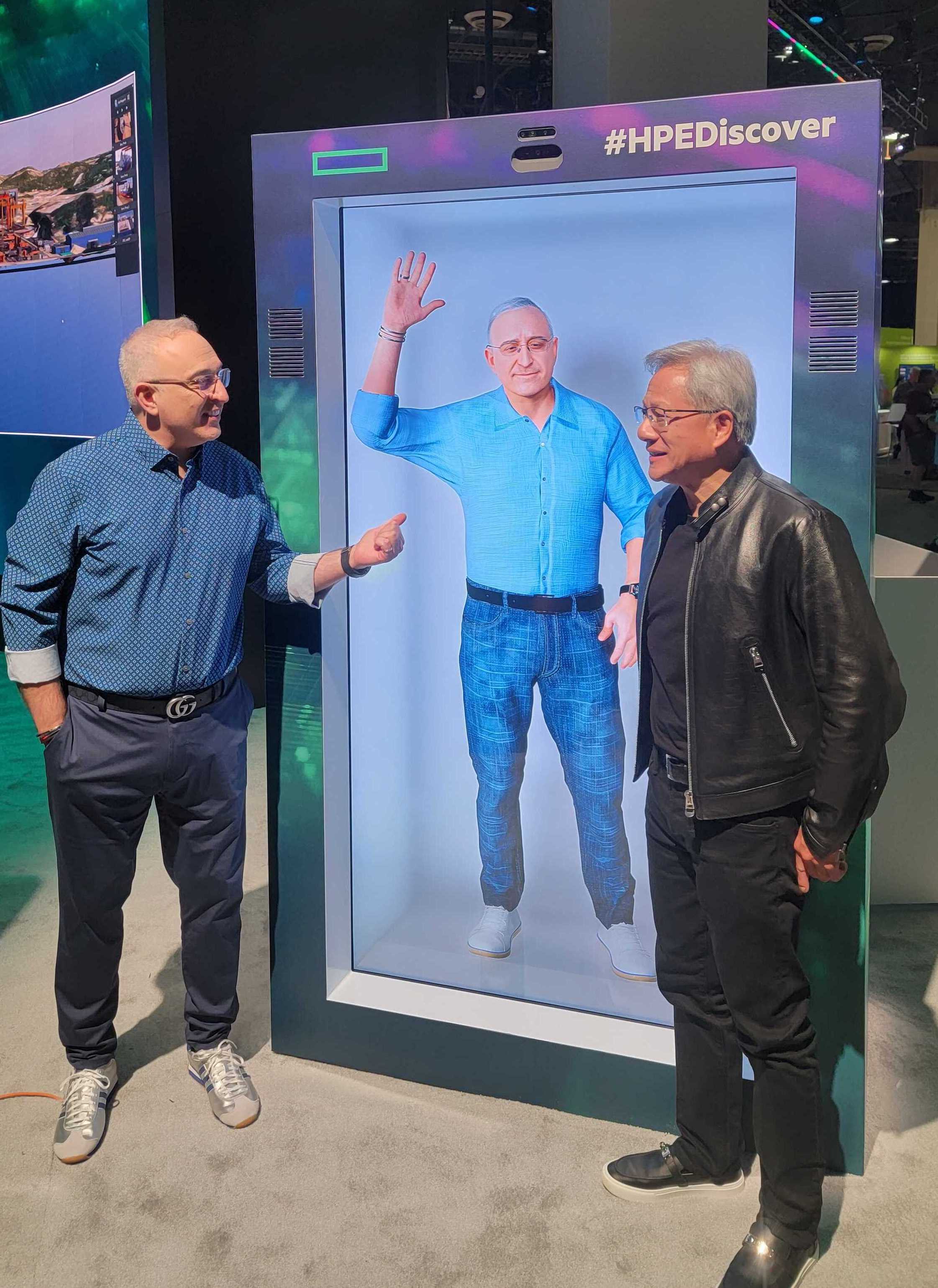
Two weeks ago at HPE Discover, the “Antonio Nearly” demo captivated the show floor, drawing the attention of Nvidia CEO Jensen Huang and HPE CEO Antonio Neri.

What is it?

Antonio Nearly is an LLM-powered holographic recreation of Antonio Neri that showcases an array of cutting-edge AI technologies. Thanks to Retrieval Augmented Generation (RAG), he’s highly knowledgeable about HPE. The powerful Llama3-70B large language model (LLM) enables him to effectively communicate this knowledge, complete with a sprinkle of witty banter. Talking to him is as simple as pressing a button and speaking into a mic, and you can ask him anything, not just HPE-related questions. Of course, because this is a representation of the CEO of HPE, we don’t want the conversation to go off the rails. That’s where the LLM guardrails kick in, ensuring that the conversation doesn’t stray into inappropriate topics. Assuming your question gets past the guardrails, the LLM (accelerated by a state-of-the-art inference server) formulates a response based on your question and any relevant documents retrieved by the RAG system. This response is quickly converted to speech using a low-latency speech synthesis model that’s finetuned to mimic the real Antonio’s voice.

Check out this video to see Antonio Nearly in action.

Why RAG?

One of the goals of this project is to enable the hologram to answer detailed, specific questions about HPE using the most up-to-date information. However, the LLM does not have the latest information, as it was trained on data from the past. While fine-tuning the LLM on newer data is an option, it is a time-consuming process and can reduce the model’s ability to generalize across diverse topics. This is particularly important because, although we want the LLM to be an expert on HPE, we also want it to be competent in discussing other subjects.

In contrast, RAG doesn’t affect the LLM’s parameters at all. Instead, a RAG system stores documents in a database that can be quickly updated with the latest information on demand. When given a question, the RAG system retrieves the most relevant documents, and passes them to the LLM. The LLM can then use the information in those documents to answer the question more effectively.

Thus, RAG is ideal for our situation where the hologram needs to be frequently updated with the latest about HPE. (For a more detailed introduction to RAG, check out our introductory blog post on the subject.)

What this blog post is about

I was fortunate to be part of the team that designed and implemented the RAG system for Antonio Nearly. So in this blog post, I’m going to explain the various components of that RAG system. Here’s what I’ll cover:

• Data sources and ingestion
• Vector DB
• Embedding model
• Reranker
• Query rephrasing
• Evaluation
• MLOps

Data sources and ingestion

Data scraping and processing

The first question is: what data do we want to put in the RAG database? Since we want the hologram to be an expert on all things HPE, our team started by scraping data from HPE blogs, press releases, and product specs.

Most of these documents touch on many different subjects, and can be quite long, making them difficult to embed in a useful way for our application. Why is that? Well, to “embed” a document means to convert the document into a vector. All documents, regardless of length, will be converted to vectors of the same length, like 384 for example. In our application, the “query document” (i.e. the user’s question for Antonio Nearly) is typically going to be 1 sentence long, and the RAG system will have to compare its embedding with the document embeddings in our database. But it is hard to effectively compare 1 sentence with a multi-page document. At the very least, it is much easier to compare 1 sentence with other documents that are also 1 sentence long.

Furthermore, embedding models have a limit on the length of the input text that they can convert into an embedding. The lightweight embedding models we are interested in simply won’t be able to process an entire multi-page document. Hence, we should aim to populate our database with relatively short documents. (Note, in the context of RAG, it’s common to refer to each entry in the database as a “document”, regardless of how much text the entry contains.)

One solution is to split long documents into smaller chunks, and store the embedding for each of these chunks. We would also store some metadata indicating that the chunk comes from the longer document, so that if the chunk is ever retrieved, we would then actually return the full document. Chunking is difficult to get right though. If you split the document in the wrong places, each chunk might not make sense on its own. If they do make sense and are retrieved as a relevant document, it still might be the case that the full document taken as a whole is not relevant.

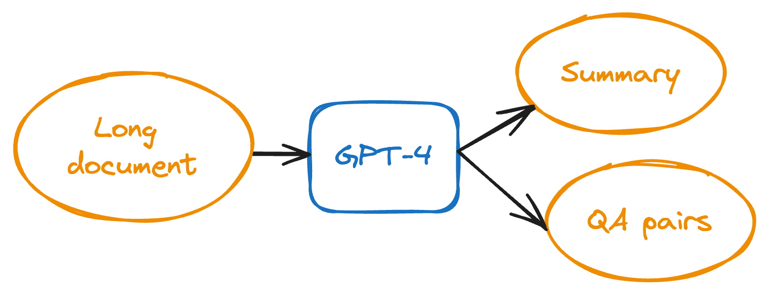
That’s why we opted for a more “GenAI” approach. For each document, we asked GPT-4 to generate a short summary and multiple question-answer (QA) pairs that relate to the content of the document. Each summary and QA pair has a very focused subject, which makes them more likely to be converted to semantically meaningful embeddings.

Embedding the documents

With the summaries and QA data in hand, the next question is how do we want to embed and store these documents? Each of our derived documents is quite short, so chunking is unnecessary. However, we do have a choice about how to embed the QA pairs. Specifically, embedding each question and answer separately could be beneficial since this further focuses the meaning of each embedding. And we don’t have to worry about the pitfalls of chunking that I mentioned above, because we know each question and answer makes sense on their own, and if a question or answer by itself is relevant to a query, so should the complete question-answer pair.

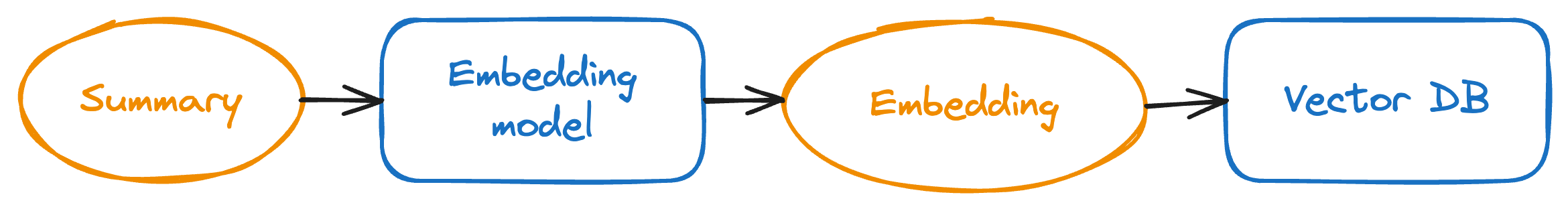
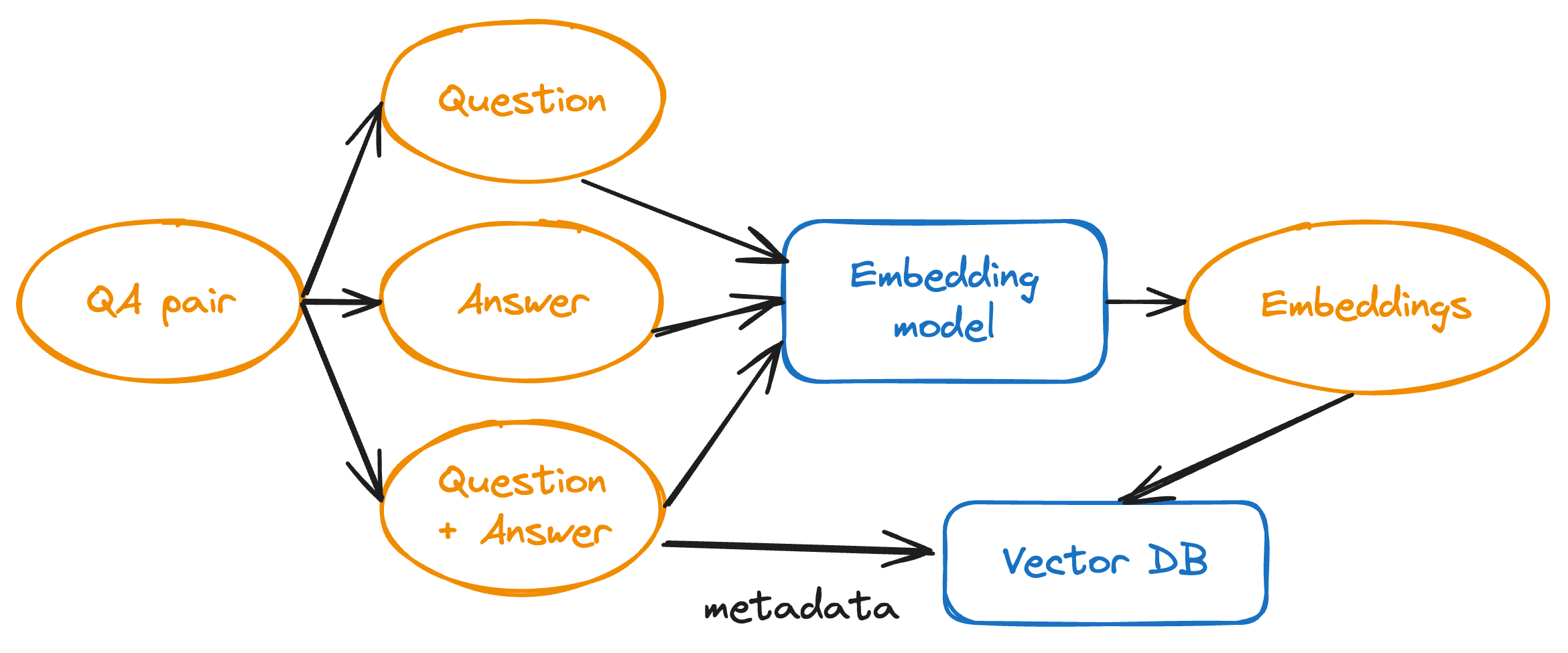
Hence, we used the following embedding strategy:

• Embed each summary as is.
• For each QA pair, embed:
  • The question by itself.
  • The answer by itself.
  • The concatenated question and answer.

  For each of these QA embeddings, we store the concatenated question-answer as metadata, and always return this metadata as the actual retrieved document. For example, if just the question embedding is retrieved, we actually return the concatenated question-answer.

Note that we are effectively embedding each QA pair three times, but from different “angles”, to reduce the chance that any relevant QA pairs are overlooked during retrieval. Also note that during retrieval, we never return any of the original multi-page documents. This is because the summaries and QA pairs are cleaner and more information-dense. Essentially, we have gotten the very powerful GPT-4 to do the heavy cognitive lifting in advance, so that we don’t have to depend entirely on the less-powerful Llama3-70B.

One special data source that the team wanted to store in the database was a spreadsheet of sessions (talks and presentations) happening at HPE Discover 2024. This spreadsheet contains data like the time, title, and description of each session, and embedding it would allow the hologram to suggest specific sessions if the user asked.

For this spreadsheet, we embedded each session in seven ways, similarly to how we embedded the QA pairs. We embedded:

• The time by itself.
• The title by itself.
• The description by itself.
• The concatenated time and title.
• The concatenated time and description.
• The concatenated title and description.
• The concatenated time, title, and description.

Like the QA pairs, we store the concatenated time, title, and description as metadata for each of the embeddings, and return the full concatenation regardless of which of the seven embeddings is retrieved.

Note that while this allows the hologram to answer questions like “Are there any sessions on AI and what time are they at?”, it doesn’t help answer aggregation questions like “How many AI sessions are there?” That would likely require a SQL integration, something we may add in the future.

Vector DB

Choice of database

A vector database stores embeddings (vectors) and their associated documents. When the RAG system receives a query (a piece of text), the query is converted into an embedding, and the vector database performs a nearest neighbor search to find the closest stored embeddings. The documents associated with these closest embeddings are assumed to be the most similar to the query.

There are many different vector databases. Some popular open-source ones include Chroma, Weaviate, Milvus, Qdrant, and Faiss. When we started the project, we chose Chroma because of its simple API and developer experience, and it seemed to provide all the features we needed. We ended up sticking with Chroma because it was convenient. Actually we didn’t do an in-depth comparison of the various vector databases, mainly because for our current demo, the database is relatively small (on the order of tens of thousands of documents), so at this scale, we figured all of them are likely to perform well and on-par with each other.

However, there were a few unexpected “gotchas” with Chroma:

• Chroma uses the HNSW library for approximate nearest neighbors search using the HNSW algorithm. One of the parameters of the HNSW algorithm is called ef, and it controls “the size of the dynamic list for the nearest neighbors”. A small ef value results in a more approximate search, and Chroma uses a default ef of 10. In other words, the default behavior of Chroma is to do a very approximate search, but this isn’t explained anywhere, even though many developers (like me) might assume that a vector database would do an exhaustive search by default. Given the small size of our database, and the importance we placed on retrieving correct information, we wanted the database to conduct as exhaustive a search as possible. This is accomplished by setting ef to the number of documents in the database.
• Chroma has an add function that takes in a list of documents, and adds them to the database. During testing, we often seed the database from scratch by adding all our documents in a single call to add. However, the add function has a size limit. If you try to add more than 41666 documents in a single add call, Chroma crashes without adding any documents to the database. This size limit isn’t explained anywhere, but it seems it has something to do with SQLite, which Chroma uses under the hood. Anyway, the workaround is to simply split the list of documents into sub-lists shorter than 41666, and call add multiple times with these sub-lists.

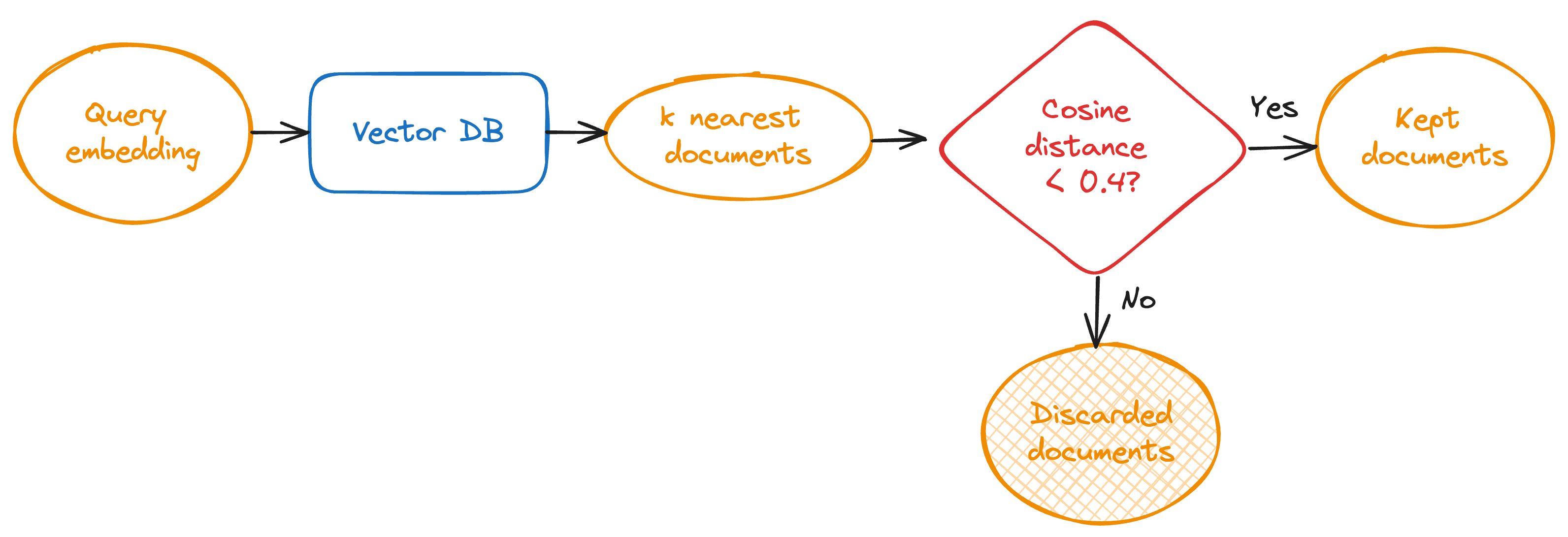
Filtering results

If we ask Chroma to return the k nearest embeddings, it will do so, regardless of how far away those embeddings are from the query document. This raises the question: should we remove results that are further than a distance d away? The upside is that if we can eliminate irrelevant results, the LLM will be less likely to get confused and bring irrelevant information into its response. The downside is that we have to somehow pick a threshold that gives us good precision and recall. In order to quantitatively evaluate this, we would need a large dataset of queries and their corresponding “correct” documents in the database. In our case, constructing a dataset like this would be particularly time-consuming (more on this in Evaluation). Ultimately, through qualitative evaluations, we settled on using a cosine distance threshold of 0.4.

Embedding model

Embedding models are what convert text to embeddings. A good embedding model will embed similar documents close together. Through qualitative evaluations we chose sentence-transformers/all-MiniLM-L12-v2 as our embedding model, which we found achieves a good balance between embedding quality and computational latency.

Reranker

As I described earlier, a vector database stores embeddings and their associated documents, and performs a nearest neighbor search to find the most relevant documents for a given query.

But there’s another way to find relevant documents. Instead of using an embedding model, which converts documents into embeddings, we could use a model that converts pairs of documents into similarity scores. This could potentially give more accurate results, because the model is basing its computations on both documents simultaneously. Cross-encoders are a type of model used for this purpose, and they do typically outperform embedding-based nearest neighbor searches. The problem is that they do not scale. For example, if we want to find a query’s most similar document among 50000 documents, we would have to pass 50000 pairs into the cross encoder to find the one with the highest similarity score.

That’s why one common approach is to first do a nearest neighbors search with the vector database, to obtain a small number of candidates, and then use a cross encoder to rerank those candidates based on its similarity scores. For example, if we limit the vector database results to 10, then we get the cross encoder to score 10 pairs. Cross encoders used in this way are called “rerankers”.

We tried using a reranking model in our pipeline, specifically BAAI/bge-reranker-base, but found that in some cases it actually made the ordering of the results worse. This plus the added latency led us to remove the reranker.

Query rephrasing

An important requirement for this project is to allow people to chat with the hologram in a casual manner, and this means being able to ask follow-up questions or refer to things previously mentioned in the conversation.

What does this mean for our RAG system? Well, let’s review what exactly our RAG system does. All documents are stored in the vector database as embeddings. So to find relevant documents, we must convert the query document into an embedding as well. The question is, what should our query document be?

• We can embed the most recent user question. This works if the question makes sense on its own, but many questions are follow-ups. For example, “Tell me more”, “What do you mean by that?”, etc. The nearest results for these follow-up questions will not be anything relevant to what the user is implicitly asking.
• We can embed the conversation history. The problem with this is that the conversation may have been predominantly about Topic A, and the user’s most recent question may be about Topic B. Thus, the embedding for the full conversation history will be more similar to Topic A than Topic B, and irrelevant documents will be retrieved.

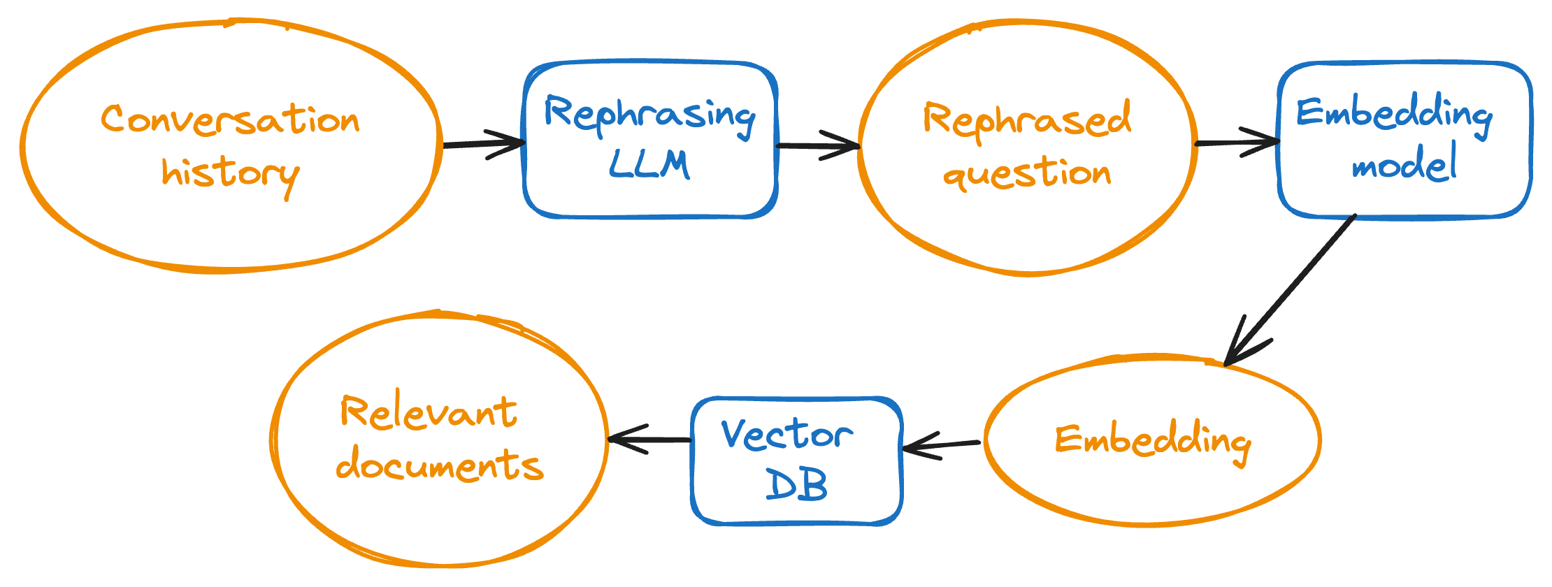
Evidently, these two options are quite flawed. Luckily, there’s a much better approach called “query rephrasing” (or “rewriting”). We feed an LLM the conversation history, ask it to rephrase the most recent user question, and use the rephrased question as our query document. (For the remainder of this post, we’ll call this LLM the “Rephrasing LLM”.) For example, given the following conversation history:

User: What is HPE GreenLake?
Assistant: <answer omitted for brevity>
User: Tell me more

the Rephrasing LLM rephrases the user’s most recent message as Can you provide more information about HPE GreenLake?

Here’s the prompt we used for the Rephrasing LLM:

Given the current conversation, rephrase the user's last 
question/request so that it makes sense without any additional 
context. Respond with only the rephrased question/request.
If no rephrasing is necessary, respond with only the original 
question/request. Do not respond with anything other than the 
rephrased or original question.

As for the Rephrasing LLM itself, we tried both Llama3-8B and Llama3-70B. The 8B was an attractive choice because latency was a big concern for this project. However, we found that we couldn’t consistently get the 8B model to follow our prompt and rephrase our question without it adding extraneous phrases like “here is your rephrased question”.

Evaluation

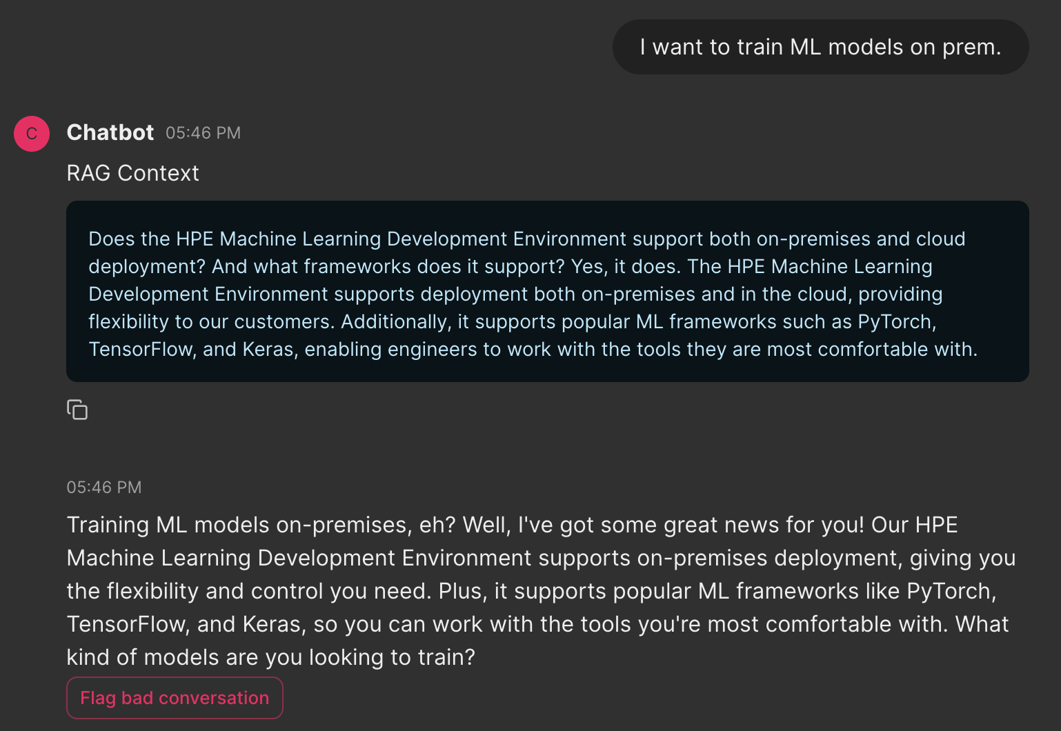
It is difficult to do a large-scale automated evaluation of a RAG system that receives conversation history, due to the many variations possible in any conversation, as well as the latency of the Rephrasing LLM. So we opted to do end-to-end qualitative tests of the LLM + Rephrasing LLM + RAG pipeline, using a Chainlit user interface (UI). The UI allows us to chat with the LLM, and it shows both the retrieved documents as well as the full prompt sent to the LLM for generating the final user-facing response. It also includes a “flag conversation” button, which flags the conversation in our logs database, to help us track failure cases.

MLOps

So far I’ve covered the more algorithmic side of the RAG system. In this final section I’ll briefly go over some of the more infrastructure-related details.

Data versioning and pipelining

Just as we version our code using git, we’d like to version our RAG data. Versioning our data is important because it enables us to reproduce performance at previous commits, roll back changes, and understand how our data affects our system’s behavior. Currently all of our data is text based, and comes in formats like csv, json, and txt. Of course, git can version this kind of text data, but we’d like to future-proof our system, and in the future we may want to support additional formats like pdf, or even multimodal data that includes images, videos, and audio. Furthermore, although our RAG system holds a relatively small amount of data, we have to remember that as we continue iterating and refining this system, we will likely add more data sources, to the point where the amount of data stored is substantial.

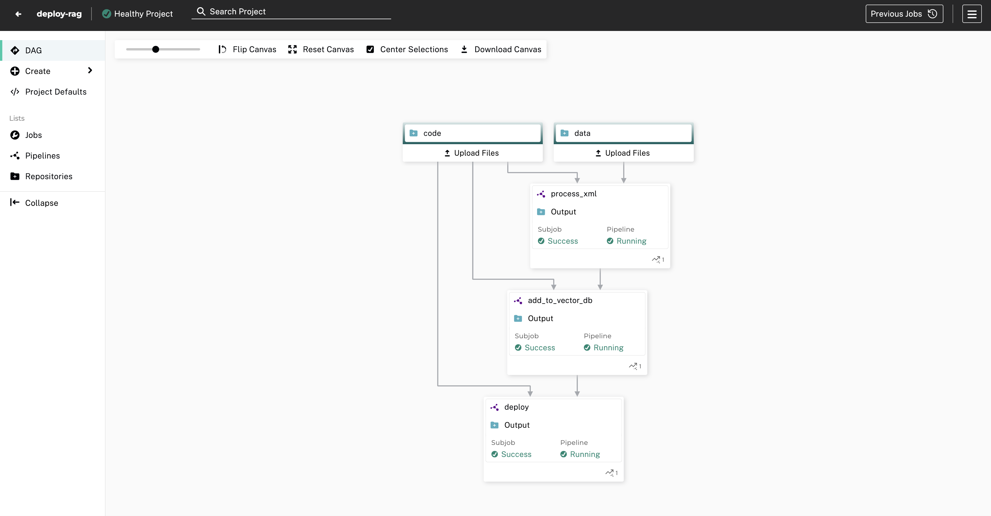
We used Pachyderm for this task, which is an open-source data versioning library that is particularly suited for large-scale unstructured data. It also takes care of pipelining, so that we can trigger actions whenever our data changes. This is ideal for a RAG system, because whenever our data repo changes, we’d like to trigger some actions like adding the new data to our vector database.

Finetuning models & containerization

There are three models in this hologram project that could be finetuned:

• The LLM that responds to the user.
• The Rephrasing LLM in the RAG system.
• The embedding model.

Finetuning large models is easy with Determined. That said, we decided not to finetune any models for this demo because we felt that improvements to other parts of the system were a higher priority.

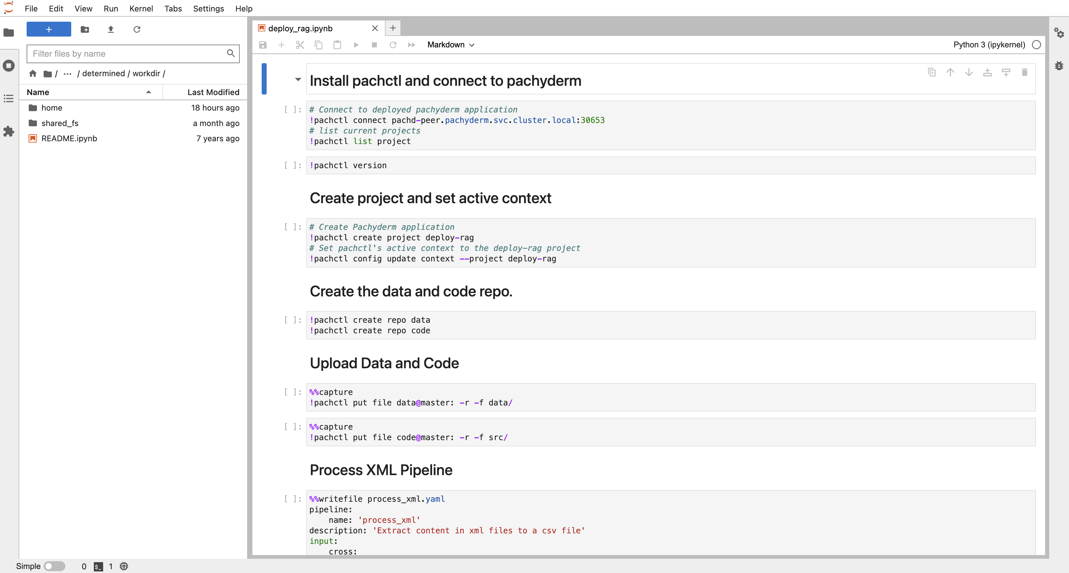
But Determined is a swiss-army knife and can be useful for more than just training models at scale. It also allows us to easily run scripts and Jupyter notebooks inside Docker containers, using an intuitive GUI. A containerized Jupyter notebook was particularly useful for us, because we wanted to interactively run Pachyderm commands inside a Docker container. This was in fact our main way of interacting with Pachyderm.

Conclusion

In this blog post, I walked through our RAG system for the Antonio Nearly hologram demo. Getting a RAG system right is challenging and requires careful attention to details and performance/latency trade-offs. It also requires understanding how the RAG system fits into the broader application.

Interested in more AI & ML content? Stay up to date by joining our Slack Community!