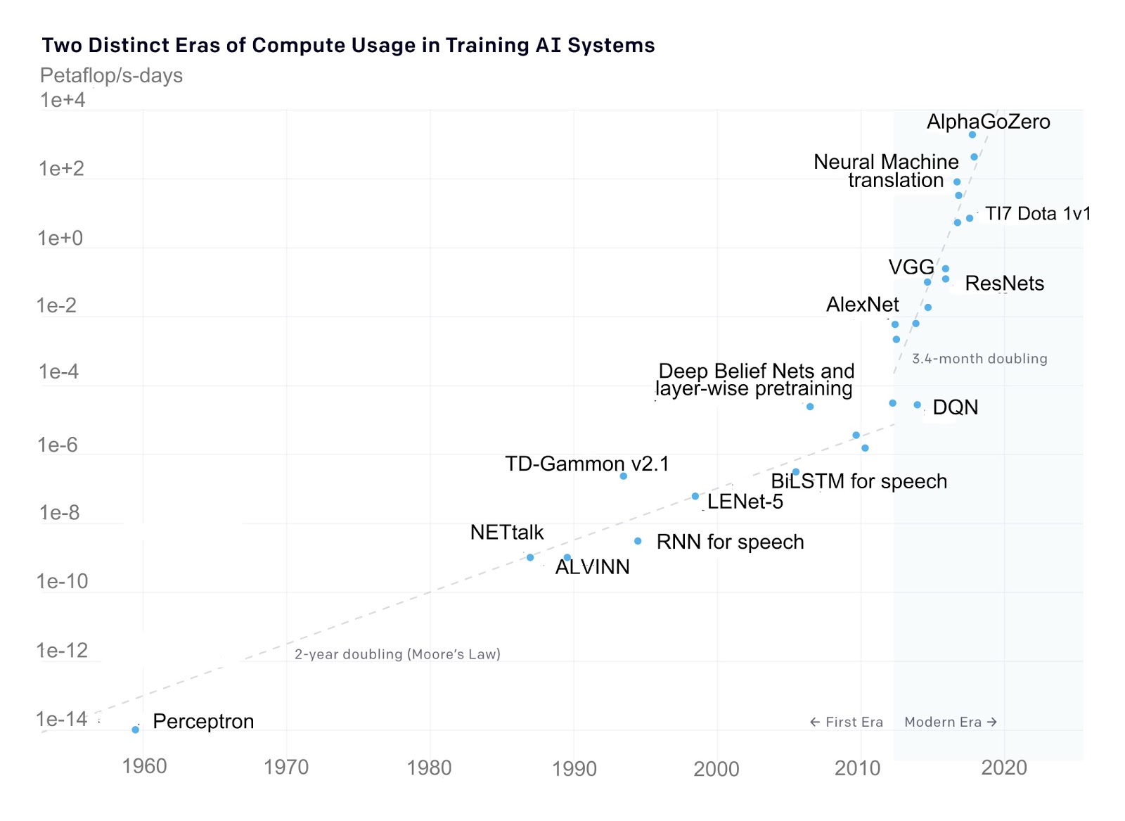
Advances in deep learning have driven tremendous progress in many industries, including autonomous driving, pharmaceutical research, and security. As deep learning models and datasets continue to grow at a pace that far exceeds the advances in computational hardware (Figure 1), distributed training functionality provided by tools like Horovod has become essential. Without the ability to train a single model with multiple GPUs at once, many modern deep learning models would take weeks to train with a single GPU!

Since being open-sourced in 2017, Horovod has continued to mature, recently graduating as an LF AI Foundation project and surpassing 10k stars on GitHub. After evaluating several distributed training tools, Determined AI chose Horovod as the foundation for the distributed training capabilities in our open-source deep learning training platform. Determined builds upon the high-performance distributed training offered by Horovod, while also providing state-of-the-art hyperparameter tuning, built-in experiment tracking, and smart scheduling and management of both on-premise and cloud GPUs.

Determined AI and the Horovod team have collaborated to improve Horovod’s performance by adding support for an optimization known as local gradient aggregation. In this post, we describe how this optimization works, present some benchmarks illustrating the performance gains it enables, and show how it can be used. Our changes to support local gradient aggregation are included in Horovod 0.21, which was released yesterday!

Faster Model Training with Local Gradient Aggregation

Horovod uses bulk-synchronous data parallelism to implement distributed training. Data parallelism works by having each worker (e.g., a GPU) load an identical copy of the model so every worker has the same model parameters. After loading the weights, training is done by applying this loop over the training data:

1. Every worker performs a forward and backward pass on a unique partition of a mini-batch of data.
2. As a result of the backward pass, every worker generates a set of updates to the model parameters based on the data it processed.
3. The workers communicate their updates to each other so that all the workers see all the updates made during that batch.
4. If averaging is enabled, every worker divides the updates by the number of workers.
5. Every worker applies the updates to its copy of the model parameters, resulting in all the workers having identical model parameters.
6. Return to step 1.

Horovod handles steps 3-5, including communicating the updates and applying them to the model parameters. The overhead of communicating the updates between workers depends on the number of workers, the interconnect between the workers (e.g., NVLink, Infiniband), the size of the model (larger models have more model parameters), and the frequency with which the communication is performed.

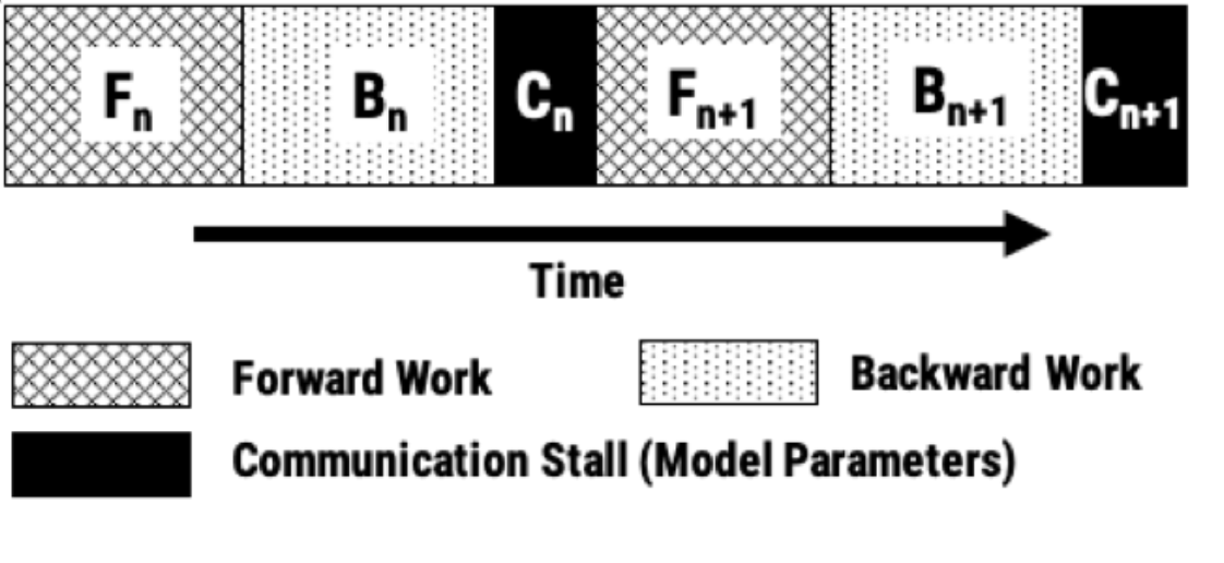
As the size of the model and the number of workers are both increased, communication often becomes the bottleneck. How can the cost of communication be reduced?

Improving the network interconnect between workers is expensive and reducing model size often comes at the tradeoff of lower accuracy. Reducing communication frequency, by increasing the amount of computation that is done per unit of communication, is typically the best approach for lowering communication overhead.

One way to reduce communication frequency is to increase the per-worker batch size, but this quickly runs into challenges: the per-worker batch size is linearly related to GPU memory consumption, so batch size per worker cannot be increased beyond the available GPU memory. Local gradient aggregation enables larger increases in effective batch size, further reducing communication overheads.

Local gradient aggregation works by having each worker perform N mini-batches (on a unique partition of the mini-batches) of work between communicating updates, where N (the aggregation frequency) is configured by the user at the start of training. During every backward pass, each worker accumulates the updates locally in GPU memory by summing the latest updates with all of the previously accumulated updates on that worker since the last round of communication. Once all workers complete N mini-batches, the local accumulated updates are communicated between workers using AllReduce resulting in all workers seeing all the updates for the last N mini-batches.

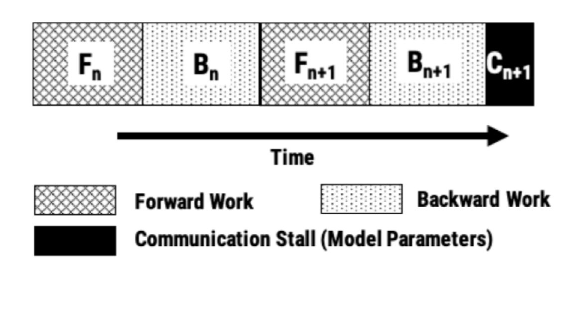
Local gradient aggregation is equivalent to using larger effective batch sizes, with workers increasing their amount of computation per unit of communication. By enabling larger effective batch sizes, local gradient aggregation reduces communication overhead by a factor of N, where N is the configured aggregation frequency. If your model training is bottlenecked by communication, enabling local gradient aggregation will improve throughput. If you aren’t sure if your model is bottlenecked by communication, try using a very high aggregation frequency (e.g., 1000); the measured speed-up will indicate your communication overhead.

Performance Benchmarks

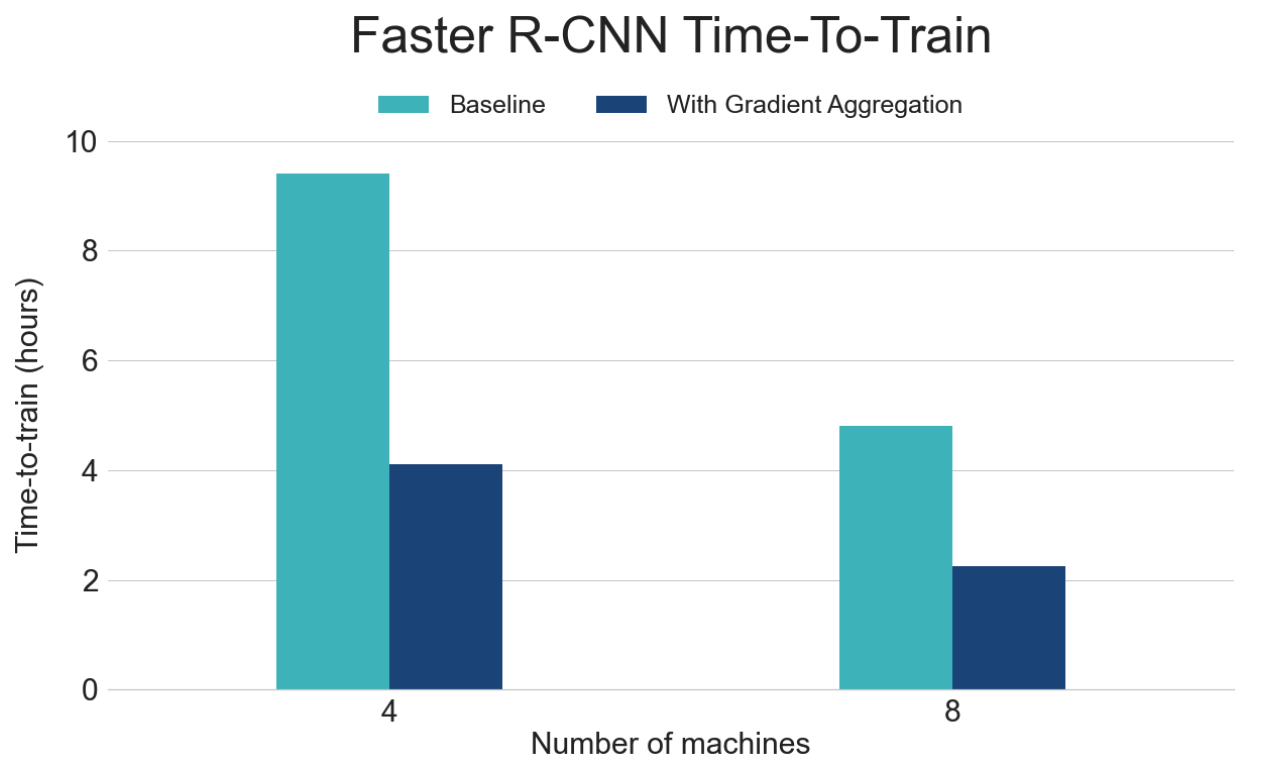
We measured the time to convergence for FasterRCNN, with and without gradient aggregation. For these benchmarks, we used a cluster of 4 and 8 machines; each machine was configured with 8 Nvidia V100 GPUs. All benchmarks use a per-GPU batch size of 1. The benchmark results are shown in Figure 4 below. Using local gradient aggregation (yellow and orange bars) significantly reduced communication overhead and shortened training time. All four configurations reached the same mAP accuracy after training for 9 epochs.

Using Local Gradient Aggregation

Configuring Gradient Aggregation in Horovod

Enabling local gradient aggregation to speed up your training is as simple as changing one flag (available in version 0.21.0 or later). When using Horovod directly all you need to do is set backward_passes_per_step to the desired aggregation frequency when initializing the Horovod optimizer:

import tensorflow as tf
from tensorflow import keras
import horovod.tensorflow.keras as hvd

# Initialize Horovod.
hvd.init()

optimizer = keras.optimizers.Adam(0.001)

# Gradient updates will be communicated every 4 mini-batches.
optimizer = hvd.DistributedOptimizer(opt, backward_passes_per_step=4)
...

Configuring Gradient Aggregation in Determined

When using Determined, switching from single-GPU training to distributed training does not require changing your model code. Instead, users simply specify the number of GPUs they want a model to be trained with, and Determined takes care of provisioning GPU instances (if necessary), scheduling the appropriate number of containers, configuring Horovod, and orchestrating distributed training. For example, to train a simple CNN on the CIFAR-10 dataset for a single epoch of data using 16 GPUs, the following experiment configuration file can be used:

description: cifar10_pytorch_distributed
hyperparameters:
  learning_rate: 1e-4
  learning_rate_decay: 1e-6
  layer1_dropout: 0.25
  layer2_dropout: 0.25
  layer3_dropout: 0.5
  global_batch_size: 512 # Per-GPU batch size of 32
resources:
  slots_per_trial: 16
records_per_epoch: 50000
searcher:
  name: single
  metric: validation_error
  max_length:
    epochs: 1
entrypoint: model_def:CIFARTrial

Enabling gradient aggregation is also just a configuration change – the aggregation frequency can be set via the optimizations.aggregation_frequency field in the experiment configuration:

optimizations:
   # Gradient updates will be communicated every 4 mini-batches.
   aggregation_frequency: 4

Next Steps

Determined makes distributed training easy! Running a distributed training job with Determined is as simple as setting a configuration parameter, as shown above: Determined takes care of provisioning the underlying hardware, scheduling the associated containers, and then uses Horovod to deliver state-of-the-art distributed training performance. Installing Determined only takes a few simple commands, and it works with both on-premise GPU clusters and in the cloud. To get started, check out the installation instructions and the quick-start guide. The Determined GitHub repo is the best place to see development activity; we’re also available to chat on Slack if you have any questions.

For more details on how to use local gradient aggregation to speed up distributed training, check out the examples in both Horovod and Determined. On the Determined AI blog, we recently discussed how local gradient aggregation can be used to speed-up fine-tuning of BERT on the SQuAD data set.

At Determined AI, we are excited to be a part of the Horovod community and hope that these optimizations allow users to continue to get better leverage on their computing resources. We believe Horovod will be a key build-blocking for scaling deep learning model development in the future.